Introduction to R: Part One

Introductions and Overview

This workshop serves as a gentle introduction to programming with R. We will cover the basics of R, such as using the command line as a calculator, working with variables, simple data structures, and data types. We will show how to load data sets into R, and how to summarize data with statistics and plots.

Opening the R command line

The R command line interface (CLI) is a simple interface for entering R commands
A command is a way of giving the computer some information and having it perform a task

Using the console as a calculator

Basic arithmetic operators

Operator	Description	Example
`+`	addition	`3 + 4 = 7`
`-`	subtraction	`10 - 2 = 8`
`*`	multiplication	`2.5 * 4 = 10`
`/`	division	`9 / 2 = 4.5`
`^`	exponentiation	`11^2 = 121`
`%%`	modulus	`5 %% 3 = 2`
`%/%`	integer division	`9 %/% 2 = 4`

# Order of operations still applies
5 - 4 + 5*2^4

## [1] 81

# Use parentheses to ensure desired order of operations
(-2 + (5 / 3.8)) * 1.618^2

## [1] -1.791211

Practice

Open up R.4.2.2. This should bring up the R welcome prompt that states what version you will be using. Next, calculate the kilograms of soil you will need to fill up a garden bed that is 1m x 2m x 1m. The density of soil is 1385 kg/m^2.

Logical operators

Logical operators test for a condition. They ask a question, and the answer is either TRUE or FALSE.

Operator	Description	Example
`<`	less than	`5 < 4 -> FALSE`
`<=`	less than or equal	`6 <= 6 -> TRUE`
`>`	greater than	`Inf > 1e6 -> TRUE`
`>=`	greater than or equal	`3.5 >= 9 -> FALSE`
`==`	exactly equal	`sin(0) == 0 -> TRUE`
`!=`	not equal	`(3+1)^2 != 3^2 + 1^1 -> TRUE`
`!`	not	`!TRUE -> FALSE`
`&&`	and (short-circuiting)	`(5 < 7) && (7 < 10) -> TRUE`
`		`
`&`	and (vectorized)	`TRUE & 2 > c(1,2,3) -> c(FALSE, FALSE, TRUE)`
`	`	or (vectorized)

Other math functions

Function	Description	Example
`abs`	absolute value of a number	`abs(-2.5), abs(3L), abs(3+4i)`
`sqrt`	square root of a number	`sqrt(0.81), sqrt(-1+0i)`
`exp`	\(e^x\)	`exp(1) ->` 2.7182818
`log`	logarithm of a number (base is the natural number \(e\) by default)
`log10`	base 10 logarithm of a number (see also `log2`, `log1p`, `logb`)
`sin`, `cos`, `tan`	basic trigonometric functions (radians by default)
`asin`, `acos`, `atan`	inverse trigonometric functions
`sinh`, `asinh`, etc.	hyperbolic and inverse hyperbolic trigonometric functions
`ceiling`	rounds a number towards infinity	`ceiling(-2.8) -> -2`
`floor`	rounds a number towards negative infinity	`floor(3.9) -> 3`
`round`	rounds a number to a specified number of digits (round to even by default)
`trunc`	strips the decimal part from a number	`trunc(2.1) -> 2`, `trunc(2.9) -> 2`

Built-in constants and other values

Keyword	Description	Example
`Inf`	The floating point representation of infinity	`1 / 0 -> Inf`
`-Inf`	Negative infinity	`1 / -0 -> -Inf`
`NaN`	Not a Number	`0 / 0 -> NaN`
`NA`	A placeholder for missing values
`NULL`	An R object representing the empty set or nothing
`pi`	The ratio of a circle’s circumference to its diameter	`3.14159...`

Using RStudio

RStudio is an integrated development environment (IDE) that provides an user-friendly environment to access your code, view graphs, get help, etc. The free desktop IDE RStudio can be downloaded here https://posit.co/downloads/.

The basic RStudio set up looks like this:

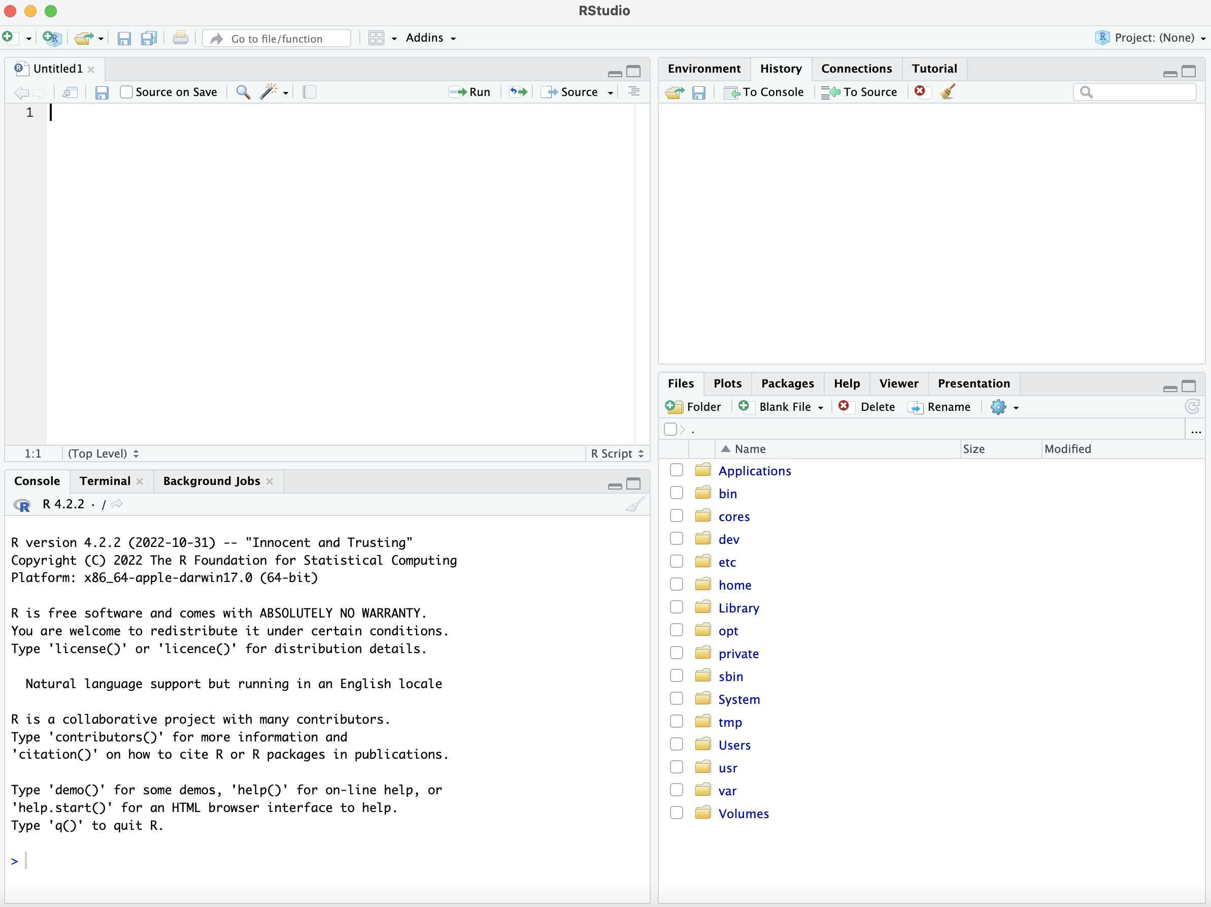
On the top left, you can create scripts. The top right shows your environment. The bottom left is your console and terminal, while the bottom right can show you the files in your working directory, the most recent plot, what packages you have downloaded, and a help menu.

How to start using RStudio

Creating projects in RStudio can help keep your data clean and reproducible. It also makes it easier to keep track of all the files, objects, and graphs you may create with your scripts. R projects can also easily be linked to Github if you are working on a collaborative project. Go to File -> New Project in RStudio. You can either create a project in a new directory (aka folder) or an existing one. For this workshop choose New Directory->R Project-> then name your folder “R_workshop”

To create a new script in RStudio you can click the icon with a white square and green check mark in the upper left hand corner of RStudio. Create a new script.

R packages

R packages are free, reproducible chunks of R code. They contain R functions, compiled code, documentation, and sometimes sample data. R packages are stored in a directory called “library” in the R environment. You can download packages using install.packages() or you can use a package like devtools or BiocManager to help the download.

install.packages("tidyverse")
if (!requireNamespace("BiocManager", quietly = TRUE))
  install.packages("BiocManager")
BiocManager::install("dada2", version = "3.16")

Accessing the built-in docs

Most if not all functions in R have useful help documentation that can be accessed directly within the R console.

help(sum)

?sum

library(help = "base")

Practice

Look at the documentation in the round() function.

What does the digits argument do?

Working with variables

Let you store a number or other object in the environment list
Similar to “memory recall” of a calculator, but better

To create a new variable, we can use <- or = assignment. Add the following code to your new script and run it:

# <- assignment
x <- 10
# = assignment
y = "abcd"

You should see both values added to the environment on the right side of RStudio
Note: The “=” for assignment is discouraged, so most people use “<-”

To list all variables in the session (environment), you can look in the environment tab in RStudio or do:

# list all variables in the environment
ls()

##  [1] "a"                      "ages"                   "billboard_raw"         
##  [4] "billboard_raw_tidy"     "cols"                   "counts"                
##  [7] "df"                     "df_patient"             "df_tidy"               
## [10] "df_treatment"           "do_first_condition"     "ends"                  
## [13] "fit"                    "huber"                  "huber_ifelse"          
## [16] "huber_vec"              "is_perfect_power"       "k"                     
## [19] "L"                      "M"                      "names"                 
## [22] "number"                 "number_of_iterations"   "pet_fct"               
## [25] "pet_obs"                "pets"                   "pew"                   
## [28] "pew_raw"                "rank"                   "read_fwf2"             
## [31] "religion"               "some_alias_for_element" "some_condition_is_true"
## [34] "some_counter"           "song"                   "starts"                
## [37] "stat"                   "t1"                     "t2"                    
## [40] "tb_clean"               "tb_raw"                 "tidy4a"                
## [43] "tidy4b"                 "values"                 "weather_clean"         
## [46] "weather_raw"            "weather_rawTest"        "x"                     
## [49] "y"                      "z"

We can see what is stored in those variables by typing them into the console:

# show what is stored in the variables
x

## [1] 10

## [1] "abcd"

Good variable naming conventions (in R)

See the tidyverse style guide for a full rundown of object naming
let your names be meaningful
let your names be consistent
avoid using existing function names (e.g. mean, c) and objects (e.g. T, F, pi)
- List of reserved words in R: https://cran.r-project.org/doc/manuals/R-lang.html#Reserved-words
avoid using dots

Basic data types in R

Data Type	Description	Example
Logical	Boolean	`TRUE or FALSE`
Integer	Whole number without decimal	`4L`
Double	Real number	`3.6`
Complex	Complex number	`3+2i`
Character	String of letters and/or numbers	`Hello 3D`

You can see what data type a variable is using the typeof() function.

Practice

What types of data are x and y?

Overview of objects and data structures

For a full overview, see the R documentation on basic types.

Vectors
Matrices and Arrays
Lists
Compound objects
- Factors
- Data frames

Working with vectors, matrices, and arrays

Vectors

a vector is a collection of same-type objects
typically created using the concatenate command, c()

# a few vectors
c(4.5, 2, 3.8)
1:4
c(TRUE, FALSE, FALSE)
seq(from = 0.1, to = 1.0, by = 0.4)
LETTERS

## [1] 4.5 2.0 3.8
## [1] 1 2 3 4
## [1]  TRUE FALSE FALSE
## [1] 0.1 0.5 0.9
##  [1] "A" "B" "C" "D" "E" "F" "G" "H" "I" "J" "K" "L" "M" "N" "O" "P" "Q" "R" "S"
## [20] "T" "U" "V" "W" "X" "Y" "Z"

We can access the elements of a vector by using brackets: []. Note that R uses “one-based indexing”, meaning that arrays start at \(1\), not \(0\).

# accessing a single element from `letters`
letters[4]

## [1] "d"

# accessing multiple elements using a vector of indices
letters[c(1, 3, 5)]

## [1] "a" "c" "e"

# accessing a subset using conditionals
x <- 1:10
x[x < 4]

## [1] 1 2 3

# accessing the last element
tail(letters, n = 1)

## [1] "z"

letters[length(letters)]

## [1] "z"

Matrices

A matrix in R is a vector with a dim attribute
It is stored in memory the same way as a vector is

# creating a matrix using the `matrix()` function
matrix(1:12, nrow = 3, ncol = 4)

##      [,1] [,2] [,3] [,4]
## [1,]    1    4    7   10
## [2,]    2    5    8   11
## [3,]    3    6    9   12

# filling a matrix with a single value
matrix("m", nrow = 5, ncol = 2)

##      [,1] [,2]
## [1,] "m"  "m" 
## [2,] "m"  "m" 
## [3,] "m"  "m" 
## [4,] "m"  "m" 
## [5,] "m"  "m"

Matrices (and vectors and arrays) are stored in column-major order

# default: fills in down each column
matrix(1:12, nrow = 3)

##      [,1] [,2] [,3] [,4]
## [1,]    1    4    7   10
## [2,]    2    5    8   11
## [3,]    3    6    9   12

# explicitly fill in accross rows first
matrix(1:12, nrow = 3, byrow = TRUE)

##      [,1] [,2] [,3] [,4]
## [1,]    1    2    3    4
## [2,]    5    6    7    8
## [3,]    9   10   11   12

Elements of a matrix can either be accessed with row-column pairs, or with linear indexing (matrix[rows, columns])

# create a 3x5 matrix
(M <- matrix(1:15, nrow = 3))

##      [,1] [,2] [,3] [,4] [,5]
## [1,]    1    4    7   10   13
## [2,]    2    5    8   11   14
## [3,]    3    6    9   12   15

# get the element at the second row and fourth column
M[2, 4]

## [1] 11

# get the 8th element in memory
M[8]

## [1] 8

Working with lists

A list is a “multi-verse” vector
Each element of a list can be any type of R object

(L <- list(a = 1, "d", formula(y ~ x)))

## $a
## [1] 1
## 
## [[2]]
## [1] "d"
## 
## [[3]]
## y ~ x

Elements of a list can be accessed in three different ways.

# Using single bracket notation. Returns a list containing the object at this index.
L[1]

## $a
## [1] 1

# Using the `$` selector. Returns the object at this index.
L$a

## [1] 1

# Using double bracket notation. Returns the object at this index.
L[[1]]

## [1] 1

Working with data frames

What are some of the key properties of a data frame?

Two dimensional (tabular)
Can be a mix of numeric, logical, and character (and more) types
All columns are the same length

A data frame is essentially a list with a few extra restrictions

Accessing elements of a data frame is similar to lists and matrices. mtcars is a dataset was extracted from the 1974 Motor Trend US magazine. The data frame is part of the base R package.

mtcars

##                      mpg cyl  disp  hp drat    wt  qsec vs am gear carb
## Mazda RX4           21.0   6 160.0 110 3.90 2.620 16.46  0  1    4    4
## Mazda RX4 Wag       21.0   6 160.0 110 3.90 2.875 17.02  0  1    4    4
## Datsun 710          22.8   4 108.0  93 3.85 2.320 18.61  1  1    4    1
## Hornet 4 Drive      21.4   6 258.0 110 3.08 3.215 19.44  1  0    3    1
## Hornet Sportabout   18.7   8 360.0 175 3.15 3.440 17.02  0  0    3    2
## Valiant             18.1   6 225.0 105 2.76 3.460 20.22  1  0    3    1
## Duster 360          14.3   8 360.0 245 3.21 3.570 15.84  0  0    3    4
## Merc 240D           24.4   4 146.7  62 3.69 3.190 20.00  1  0    4    2
## Merc 230            22.8   4 140.8  95 3.92 3.150 22.90  1  0    4    2
## Merc 280            19.2   6 167.6 123 3.92 3.440 18.30  1  0    4    4
## Merc 280C           17.8   6 167.6 123 3.92 3.440 18.90  1  0    4    4
## Merc 450SE          16.4   8 275.8 180 3.07 4.070 17.40  0  0    3    3
## Merc 450SL          17.3   8 275.8 180 3.07 3.730 17.60  0  0    3    3
## Merc 450SLC         15.2   8 275.8 180 3.07 3.780 18.00  0  0    3    3
## Cadillac Fleetwood  10.4   8 472.0 205 2.93 5.250 17.98  0  0    3    4
## Lincoln Continental 10.4   8 460.0 215 3.00 5.424 17.82  0  0    3    4
## Chrysler Imperial   14.7   8 440.0 230 3.23 5.345 17.42  0  0    3    4
## Fiat 128            32.4   4  78.7  66 4.08 2.200 19.47  1  1    4    1
## Honda Civic         30.4   4  75.7  52 4.93 1.615 18.52  1  1    4    2
## Toyota Corolla      33.9   4  71.1  65 4.22 1.835 19.90  1  1    4    1
## Toyota Corona       21.5   4 120.1  97 3.70 2.465 20.01  1  0    3    1
## Dodge Challenger    15.5   8 318.0 150 2.76 3.520 16.87  0  0    3    2
## AMC Javelin         15.2   8 304.0 150 3.15 3.435 17.30  0  0    3    2
## Camaro Z28          13.3   8 350.0 245 3.73 3.840 15.41  0  0    3    4
## Pontiac Firebird    19.2   8 400.0 175 3.08 3.845 17.05  0  0    3    2
## Fiat X1-9           27.3   4  79.0  66 4.08 1.935 18.90  1  1    4    1
## Porsche 914-2       26.0   4 120.3  91 4.43 2.140 16.70  0  1    5    2
## Lotus Europa        30.4   4  95.1 113 3.77 1.513 16.90  1  1    5    2
## Ford Pantera L      15.8   8 351.0 264 4.22 3.170 14.50  0  1    5    4
## Ferrari Dino        19.7   6 145.0 175 3.62 2.770 15.50  0  1    5    6
## Maserati Bora       15.0   8 301.0 335 3.54 3.570 14.60  0  1    5    8
## Volvo 142E          21.4   4 121.0 109 4.11 2.780 18.60  1  1    4    2

# getting a single column using the `$` selector or `[[`
mtcars$mpg # column "mpg"

##  [1] 21.0 21.0 22.8 21.4 18.7 18.1 14.3 24.4 22.8 19.2 17.8 16.4 17.3 15.2 10.4
## [16] 10.4 14.7 32.4 30.4 33.9 21.5 15.5 15.2 13.3 19.2 27.3 26.0 30.4 15.8 19.7
## [31] 15.0 21.4

#mtcars[["mpg"]] # column "mpg"
# getting multiple columns using `[` and a index/character vector
mtcars["mpg"] # a new data frame with just the "mpg" column

##                      mpg
## Mazda RX4           21.0
## Mazda RX4 Wag       21.0
## Datsun 710          22.8
## Hornet 4 Drive      21.4
## Hornet Sportabout   18.7
## Valiant             18.1
## Duster 360          14.3
## Merc 240D           24.4
## Merc 230            22.8
## Merc 280            19.2
## Merc 280C           17.8
## Merc 450SE          16.4
## Merc 450SL          17.3
## Merc 450SLC         15.2
## Cadillac Fleetwood  10.4
## Lincoln Continental 10.4
## Chrysler Imperial   14.7
## Fiat 128            32.4
## Honda Civic         30.4
## Toyota Corolla      33.9
## Toyota Corona       21.5
## Dodge Challenger    15.5
## AMC Javelin         15.2
## Camaro Z28          13.3
## Pontiac Firebird    19.2
## Fiat X1-9           27.3
## Porsche 914-2       26.0
## Lotus Europa        30.4
## Ford Pantera L      15.8
## Ferrari Dino        19.7
## Maserati Bora       15.0
## Volvo 142E          21.4

mtcars[1:3] # columns 1 through 3

##                      mpg cyl  disp
## Mazda RX4           21.0   6 160.0
## Mazda RX4 Wag       21.0   6 160.0
## Datsun 710          22.8   4 108.0
## Hornet 4 Drive      21.4   6 258.0
## Hornet Sportabout   18.7   8 360.0
## Valiant             18.1   6 225.0
## Duster 360          14.3   8 360.0
## Merc 240D           24.4   4 146.7
## Merc 230            22.8   4 140.8
## Merc 280            19.2   6 167.6
## Merc 280C           17.8   6 167.6
## Merc 450SE          16.4   8 275.8
## Merc 450SL          17.3   8 275.8
## Merc 450SLC         15.2   8 275.8
## Cadillac Fleetwood  10.4   8 472.0
## Lincoln Continental 10.4   8 460.0
## Chrysler Imperial   14.7   8 440.0
## Fiat 128            32.4   4  78.7
## Honda Civic         30.4   4  75.7
## Toyota Corolla      33.9   4  71.1
## Toyota Corona       21.5   4 120.1
## Dodge Challenger    15.5   8 318.0
## AMC Javelin         15.2   8 304.0
## Camaro Z28          13.3   8 350.0
## Pontiac Firebird    19.2   8 400.0
## Fiat X1-9           27.3   4  79.0
## Porsche 914-2       26.0   4 120.3
## Lotus Europa        30.4   4  95.1
## Ford Pantera L      15.8   8 351.0
## Ferrari Dino        19.7   6 145.0
## Maserati Bora       15.0   8 301.0
## Volvo 142E          21.4   4 121.0

Practice !

On your script make a variable “age” that is populated by your age, a vector named “favorite_foods” with at least 3 foods, and list that holds the times you have class on Mondays and Fridays.

What the name of the 8th column of the mtcar data table?

Fitting a linear model

R has built-in support for fitting generalized linear models, with support for numeric and factor variables.

x <- rnorm(30)
y <- rnorm(length(x), 3*x + 2, 0.5)
# fit a linear model
lm(y ~ x) # slope-intercept model. Same as `lm(y ~ 1 + x)`

## 
## Call:
## lm(formula = y ~ x)
## 
## Coefficients:
## (Intercept)            x  
##       2.046        2.959

lm(y ~ 0 + x) # slope only model (no intercept)

## 
## Call:
## lm(formula = y ~ 0 + x)
## 
## Coefficients:
##     x  
## 3.426

Practice time!

Write a script that creates a linear model relating mpg and cyl of the mtcars data frame.

What is the y intercept for your linear model?
How can you set the y intercept to 0? When would you want to do this?

Calling Data, Functions, and a little about Tidyverse, and reproducible data

In this section we will go over how to bring in datasets from online, spreadsheets, or another statistical program like SPSS. We will also briefly talk about functions, using a library called tidyverse, and some aspects of reproducible data.Common data files include .csv, .txt, or .xlsx, which all can be uploaded into R.

Download a file from the internet

Here is an example of how to downloaded a csv from the Nevada INBRE github page and we specify the new file name.

download.file(url="https://raw.githubusercontent.com/NevadaINBRE/NevadaINBRE.github.io/main/docs/data/billboard.csv", 
              destfile =  "my_tmp_NewBillboard.csv")

Read in data from the internet (rather than downloading)

With the package readr we can directly read in data from the internet rather than downloading it onto the local computer.

library (readr)

url_location <- "https://raw.githubusercontent.com/NevadaINBRE/NevadaINBRE.github.io/main/docs/data/billboard.csv"
suppressMessages(myBillboard <- read_csv(url(url_location)))

Read in data from the local computer

Let’s use the file we downloaded and read it in

myOtherBillboard <- read.csv("my_tmp_NewBillboard.csv")

After reading in data, it is good practice to check what the data look like within the R environment. There are multiple ways to do that:

head(myBillboard)

## # A tibble: 6 × 83
##    year artist.inverted     track time  genre date.entered date.peaked x1st.week
##   <dbl> <chr>               <chr> <tim> <chr> <date>       <date>          <dbl>
## 1  2000 Destiny's Child     Inde… 03:38 Rock  2000-09-23   2000-11-18         78
## 2  2000 Santana             Mari… 04:18 Rock  2000-02-12   2000-04-08         15
## 3  2000 Savage Garden       I Kn… 04:07 Rock  1999-10-23   2000-01-29         71
## 4  2000 Madonna             Music 03:45 Rock  2000-08-12   2000-09-16         41
## 5  2000 Aguilera, Christina Come… 03:38 Rock  2000-08-05   2000-10-14         57
## 6  2000 Janet               Does… 04:17 Rock  2000-06-17   2000-08-26         59
## # ℹ 75 more variables: x2nd.week <dbl>, x3rd.week <dbl>, x4th.week <dbl>,
## #   x5th.week <dbl>, x6th.week <dbl>, x7th.week <dbl>, x8th.week <dbl>,
## #   x9th.week <dbl>, x10th.week <dbl>, x11th.week <dbl>, x12th.week <dbl>,
## #   x13th.week <dbl>, x14th.week <dbl>, x15th.week <dbl>, x16th.week <dbl>,
## #   x17th.week <dbl>, x18th.week <dbl>, x19th.week <dbl>, x20th.week <dbl>,
## #   x21st.week <dbl>, x22nd.week <dbl>, x23rd.week <dbl>, x24th.week <dbl>,
## #   x25th.week <dbl>, x26th.week <dbl>, x27th.week <dbl>, x28th.week <dbl>, …

head(myOtherBillboard)

##   year     artist.inverted                                 track time genre
## 1 2000     Destiny's Child              Independent Women Part I 3:38  Rock
## 2 2000             Santana                          Maria, Maria 4:18  Rock
## 3 2000       Savage Garden                    I Knew I Loved You 4:07  Rock
## 4 2000             Madonna                                 Music 3:45  Rock
## 5 2000 Aguilera, Christina Come On Over Baby (All I Want Is You) 3:38  Rock
## 6 2000               Janet                 Doesn't Really Matter 4:17  Rock
##   date.entered date.peaked x1st.week x2nd.week x3rd.week x4th.week x5th.week
## 1   2000-09-23  2000-11-18        78        63        49        33        23
## 2   2000-02-12  2000-04-08        15         8         6         5         2
## 3   1999-10-23  2000-01-29        71        48        43        31        20
## 4   2000-08-12  2000-09-16        41        23        18        14         2
## 5   2000-08-05  2000-10-14        57        47        45        29        23
## 6   2000-06-17  2000-08-26        59        52        43        30        29
##   x6th.week x7th.week x8th.week x9th.week x10th.week x11th.week x12th.week
## 1        15         7         5         1          1          1          1
## 2         3         2         2         1          1          1          1
## 3        13         7         6         4          4          4          6
## 4         1         1         1         1          2          2          2
## 5        18        11         9         9         11          1          1
## 6        22        15        10        10          5          1          1
##   x13th.week x14th.week x15th.week x16th.week x17th.week x18th.week x19th.week
## 1          1          1          1          1          1          1          1
## 2          1          1          1          1          1          1          8
## 3          4          2          1          1          1          2          1
## 4          2          2          4          8         11         16         20
## 5          1          1          4          8         12         22         23
## 6          1          2          2          3          3          7          8
##   x20th.week x21st.week x22nd.week x23rd.week x24th.week x25th.week x26th.week
## 1          2          3          7         10         12         15         22
## 2         15         19         21         26         36         48         47
## 3          2          4          8          8         12         14         17
## 4         25         27         27         29         44         NA         NA
## 5         43         44         NA         NA         NA         NA         NA
## 6         20         25         37         40         41         NA         NA
##   x27th.week x28th.week x29th.week x30th.week x31st.week x32nd.week x33rd.week
## 1         29         31         NA         NA         NA         NA         NA
## 2         NA         NA         NA         NA         NA         NA         NA
## 3         21         24         30         34         37         46         47
## 4         NA         NA         NA         NA         NA         NA         NA
## 5         NA         NA         NA         NA         NA         NA         NA
## 6         NA         NA         NA         NA         NA         NA         NA
##   x34th.week x35th.week x36th.week x37th.week x38th.week x39th.week x40th.week
## 1         NA         NA         NA         NA         NA         NA         NA
## 2         NA         NA         NA         NA         NA         NA         NA
## 3         NA         NA         NA         NA         NA         NA         NA
## 4         NA         NA         NA         NA         NA         NA         NA
## 5         NA         NA         NA         NA         NA         NA         NA
## 6         NA         NA         NA         NA         NA         NA         NA
##   x41st.week x42nd.week x43rd.week x44th.week x45th.week x46th.week x47th.week
## 1         NA         NA         NA         NA         NA         NA         NA
## 2         NA         NA         NA         NA         NA         NA         NA
## 3         NA         NA         NA         NA         NA         NA         NA
## 4         NA         NA         NA         NA         NA         NA         NA
## 5         NA         NA         NA         NA         NA         NA         NA
## 6         NA         NA         NA         NA         NA         NA         NA
##   x48th.week x49th.week x50th.week x51st.week x52nd.week x53rd.week x54th.week
## 1         NA         NA         NA         NA         NA         NA         NA
## 2         NA         NA         NA         NA         NA         NA         NA
## 3         NA         NA         NA         NA         NA         NA         NA
## 4         NA         NA         NA         NA         NA         NA         NA
## 5         NA         NA         NA         NA         NA         NA         NA
## 6         NA         NA         NA         NA         NA         NA         NA
##   x55th.week x56th.week x57th.week x58th.week x59th.week x60th.week x61st.week
## 1         NA         NA         NA         NA         NA         NA         NA
## 2         NA         NA         NA         NA         NA         NA         NA
## 3         NA         NA         NA         NA         NA         NA         NA
## 4         NA         NA         NA         NA         NA         NA         NA
## 5         NA         NA         NA         NA         NA         NA         NA
## 6         NA         NA         NA         NA         NA         NA         NA
##   x62nd.week x63rd.week x64th.week x65th.week x66th.week x67th.week x68th.week
## 1         NA         NA         NA         NA         NA         NA         NA
## 2         NA         NA         NA         NA         NA         NA         NA
## 3         NA         NA         NA         NA         NA         NA         NA
## 4         NA         NA         NA         NA         NA         NA         NA
## 5         NA         NA         NA         NA         NA         NA         NA
## 6         NA         NA         NA         NA         NA         NA         NA
##   x69th.week x70th.week x71st.week x72nd.week x73rd.week x74th.week x75th.week
## 1         NA         NA         NA         NA         NA         NA         NA
## 2         NA         NA         NA         NA         NA         NA         NA
## 3         NA         NA         NA         NA         NA         NA         NA
## 4         NA         NA         NA         NA         NA         NA         NA
## 5         NA         NA         NA         NA         NA         NA         NA
## 6         NA         NA         NA         NA         NA         NA         NA
##   x76th.week
## 1         NA
## 2         NA
## 3         NA
## 4         NA
## 5         NA
## 6         NA

tail(myBillboard)

## # A tibble: 6 × 83
##    year artist.inverted  track    time  genre date.entered date.peaked x1st.week
##   <dbl> <chr>            <chr>    <tim> <chr> <date>       <date>          <dbl>
## 1  2000 Master P         Souljas  03:33 Rap   2000-11-18   2000-11-18         98
## 2  2000 Ghostface Killah Cherche… 03:04 R&B   2000-08-05   2000-08-05         98
## 3  2000 Smith, Will      Freakin… 03:58 Rap   2000-02-12   2000-02-12         99
## 4  2000 Zombie Nation    Kernkra… 03:30 Rock  2000-09-02   2000-09-02         99
## 5  2000 Eastsidaz, The   Got Beef 03:58 Rap   2000-07-01   2000-07-01         99
## 6  2000 Fragma           Toca's … 03:22 R&B   2000-10-28   2000-10-28         99
## # ℹ 75 more variables: x2nd.week <dbl>, x3rd.week <dbl>, x4th.week <dbl>,
## #   x5th.week <dbl>, x6th.week <dbl>, x7th.week <dbl>, x8th.week <dbl>,
## #   x9th.week <dbl>, x10th.week <dbl>, x11th.week <dbl>, x12th.week <dbl>,
## #   x13th.week <dbl>, x14th.week <dbl>, x15th.week <dbl>, x16th.week <dbl>,
## #   x17th.week <dbl>, x18th.week <dbl>, x19th.week <dbl>, x20th.week <dbl>,
## #   x21st.week <dbl>, x22nd.week <dbl>, x23rd.week <dbl>, x24th.week <dbl>,
## #   x25th.week <dbl>, x26th.week <dbl>, x27th.week <dbl>, x28th.week <dbl>, …

View(myBillboard)
myBillboard[1:4,1:4]

## # A tibble: 4 × 4
##    year artist.inverted track                    time  
##   <dbl> <chr>           <chr>                    <time>
## 1  2000 Destiny's Child Independent Women Part I 03:38 
## 2  2000 Santana         Maria, Maria             04:18 
## 3  2000 Savage Garden   I Knew I Loved You       04:07 
## 4  2000 Madonna         Music                    03:45

dim(myBillboard)

## [1] 317  83

dim(myOtherBillboard)

## [1] 317  83

There are many other functions to read in data, but we can also read in an objects. Two common R object are .rds and .RData. We will have an example of this later.

Writing functions

We’ve already seen some functions like abs() or type()
Packages are usually compilations of functions
Functions are necessary to write flexible and reusable code
Rule of thumb: if you copy and paste a block of code more than once, turn it into a function
- this applies to making plots as well
Functions are made up of 3 components
- Body: The code inside a function
- Formals, aka input: A list of arguments that controls how you call a function
- Environment: A map of where the variables of the function are located

Functions usually look like this:

function_example <- function(formals){
  body_of_function 
  }

Let’s build a function that calculates the mean of four input variables:

my_mean_fun <- function(x1, x2, x3, x4){
  my_mean <- (x1 + x2 + x3 + x4)/4 
  }